DMN is not optimized for machine learning algorithms, but it's good enough for simple problems such as fitting a straight line to a set of data points, known as linear regression. In this post we'll look at two ways to do it.
Consider the table Dataset, a list of x-y pairs. Here x represents the number of members in a group health insurance plan, and y represents the administrative cost of the plan as a percentage of claim value. We would expect the admin cost percentage to decrease as the number of members increases, which is what we see when we graph the table.
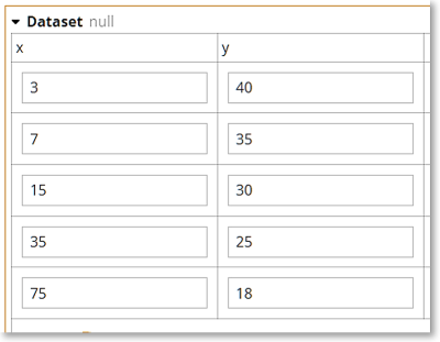
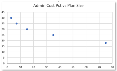
Here we have 6 data points {x[i], y[i]}, and we want to find the best straight line fit, described as
y = m*x + bwhere m is the slope of the line and b is the intercept of the line at x = 0, using linear regression.
Best fit means minimizing the sum of the square of errors, where error is the actual y value minus the straight line y value. When the dependent variable y depends only on a single variable x, we can find the best fit analytically. When there are additional independent variables, we typically need to use numerical methods.
Analytical Solution
Using the analytical solution, the slope m is given by(n*sumxy – sumx*sumy)/(n*sumx2 – sumx**2)and b is given by
(sumy – m*sumx)/nwhere
n = count(Dataset)sumxy = sum(for i in 1..n return Dataset.x[i]*Dataset.y[i])sumx = sum(Dataset.x)sumy = sum(Dataset.y)sumx2 = sum(for i in 1..n return Dataset.x[i]**2)
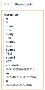
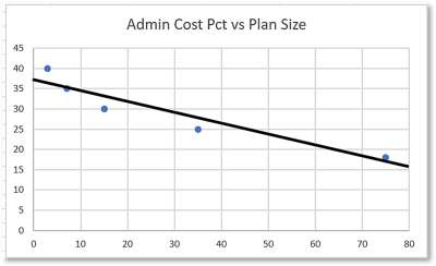
OK, it's good to know how to do this, but it's not all that profound. More interesting is the case where we do not have an analytical solution and we need to do it another way.
Numerical Solution Using Gradient Descent
When the dependent variable y is a linear expression of multiple variables, we must resort to numerical methods to estimate the coefficients of each independent variable that minimize the cost function, the sum of the squared difference between the modeled value and the observed or actual value.One common way to do this is called gradient descent. We calculate the cost function for some initial guess at the coefficients, then iteratively adjust the coefficients and calculate the cost function again until it approaches a minimum. The adjustment is based on the gradient of the cost function, meaning the slope of the cost function curve when you vary one coefficient while keeping the other values constant. Doing this successfully depends on the proper choice of a parameter called the learning rate. If you set the learning rate too high, the iterations do not converge on a minimum; if you set it too low, it will converge but could take thousands of iterations.
Gradient descent is used in many machine learning algorithms besides linear regression, including classification using logistic regression, even neural networks. But here we will see how it works with linear regression using the same dataset we used previously.
We calculate the cost function in FEEL as
cost = sum(for i in 1..n return (h[i] – y[i])**2)/(2*n)where h[i] is the estimated value of y[i]. In the case of linear regression,
h[i] = c1*x[i] + c0where c1 and c0 are the coefficients we are trying to optimize. If we are successful they will equal the values of m and b calculated previously.
Gradient descent means we adjust our initial guess of the coefficients by multiplying the learning rate a times the partial derivative of the cost function with respect to each coefficient. The adjustment with each iteration is given by
c0 := c0 – a/n*sum(for i in 1..n return h[i] – y[i])
c1 := c1 – a/n*sum(for i in 1..n return x[i]*(h[i] – y[i]) To do this in DMN requires recursion, a function that calls itself with new arguments each time. Each iteration generates new values for c0 and c1, from which we calculate cost, and we iterate until cost converges on a minimum.
When we use the raw Dataset values, we need to set the learning rate to a very small number, and it requires too many iterations to converge to the minimum cost. We can get much faster convergence is by normalizing the data:
xn[i] = (x[i] – xmin)/(xmax – xmin)
yn[i] = (y[i] – ymin)/(ymax – ymin) Now the normalized values xn and yn all lie in the interval [0..1]. We can use gradient descent on the normalized dataset to find values of cn0 and cn1 that minimize the cost function for the regression line
yn = cn1*xn + cn0and then transform the coefficients to get c0 and c1, which apply to the raw Dataset.
The DRD for our model is shown below:
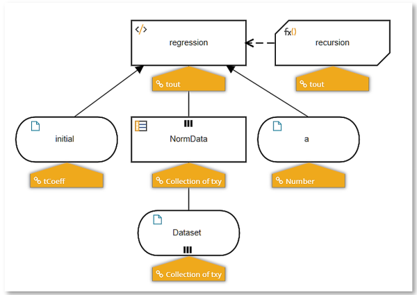
Decision NormData applies the normalization transformation to the raw Dataset. Input data initial is our initial guess at the coefficients, which we naively set to cn1=0, cn0=0. We play around with the learning rate a until we find one that converges well. The decision regression calls the BKM recursion once, with the initial coefficient values. The BKM calculates the cost function, adjusts values of the coefficients, and then iteratively calls itself again with the new coefficients.
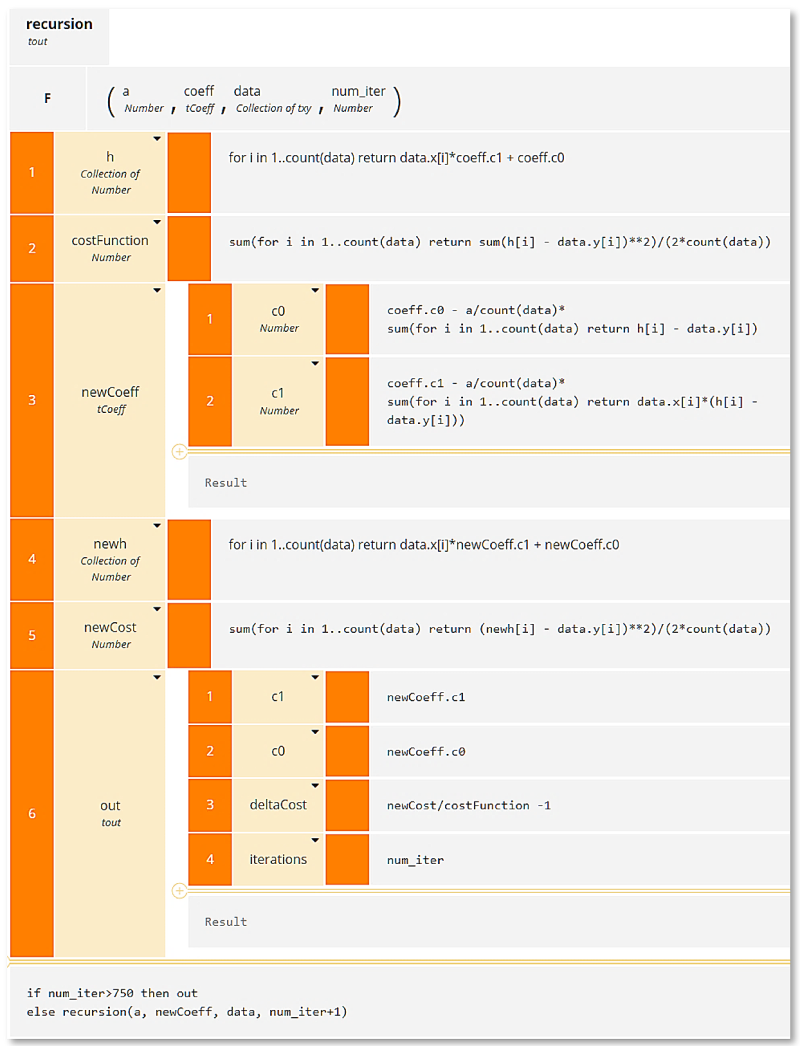
In the BKM, context entry h is the collection of estimated y values using the coefficients specified by the BKM parameter coeff. Context entry costFunction is the calculated cost using h. Context entry newCoeff uses the gradient descent formula with learning rate a to generate new coefficient values. From that we calculate new values of h and a new value for the cost function.
We can set recursion to end at a certain number of iterations or when the cost function change is essentially zero. In the final result box, we recursively call the BKM 750 times with adjusted coefficient values. Context entry out is the structure output by the BKM when we exit. It provides values for the coefficients, the fractional change in the cost function from the previous iteration – ideally near zero, and the count of iterations.
Executing this model with initial guess {c0:0, c1:0} for the coefficients and 0.1 for the learning rate a, we get the result below:
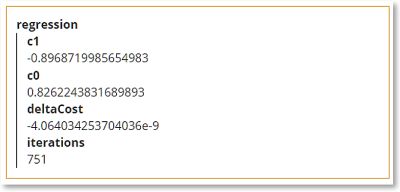
Convergence is excellent; after 750 iterations the fractional change in the cost function is a few parts per billion. Now we need to convert the coefficients – here labeled c1 and c0 but actually what we earlier called cn1 and cn0 – to the c1 and c0 values for the raw Dataset.
Plugging the calculated values of -0.897 for cn1 and 0.826 for cn0 into the normalization equations
-
yn = cn1*xn + cn0
-
xn = (x – xmin)/(xmax – xmin)
-
yn = (y – ymin)/(ymax – ymin)
-
y = c1*x + c0
You would likely use the analytical solution, not gradient descent, for linear regression on a single variable, but for many other machine learning problems, numerical methods for minimizing the cost function are the only way. To be fair, many other languages do this more easily than DMN, but if you need to sneak in a bit of machine learning to your DMN model, you can do it!
These examples, along with many others, are taken from the DMN Cookbook section of my new book, DMN Method and Style 3rd edition, coming soon.
