DMN is excellent at working with tables of data. Such a table in DMN is called a relation. A relation is defined as a list of rows with a specific number of named columns. The number of rows in a DMN relation is unspecified. Most decision models work with tables in this form.
But what if you want your DMN model to work with numeric tables having an unspecified number of columns and rows? In DMN that is not a relation. It is a matrix. In a matrix, the cells have numeric values, the columns are unnamed, and there can be any number of them. In DMN, a matrix is modeled as a list of number lists.
Some decision models involving tables of data can be implemented either using relations or matrices. While some FEEL expressions are simpler using relations, matrices have the advantage that the decision logic does not depend on the number or names of the columns. That means you can use the same decision model with tables with different numbers of columns. Also, in some cases the decision logic is simpler using matrices than the equivalent relation. For example, using relations, mapping table T1, with columns c1, c2, and c3, to table T2 of the same type requires a context with a context entry for each component and a cell expression for each one. With matrices, it requires just a literal expression involving iteration.
Manipulating matrices in FEEL is a little tricky, but in this post we’ll see how to do it.
Relations vs Matrices
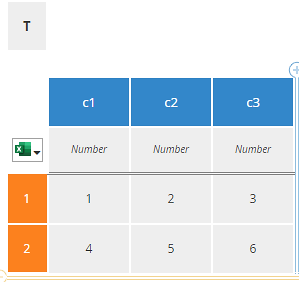
To illustrate the difference between a DMN relation and a matrix construct, consider T, a table with columns named c1, c2, and c3. T is a DMN relation. Each row of T is defined as a data structure with named components representing the columns of T. The datatype of the row – let’s call it tRow – specifies those components. Since T is a list of rows, the datatype of the table T – let’s call it tTable – is a collection of tRow.The rows of T do not have names; they are referenced by number, modeled as an index enclosed in square brackets. T[1] means the first row of the table. The columns of T have specific names, for example, c1, c2, and c3. Models involving elements of T need to specifically reference c1, c2, and c3 by name. You cannot reference them by number, e.g. the second column. For example, in FEEL the column c2 is simply T.c2. Cell c2 of the first row is either T[1].c2 or T.c2[1]. Both have the same value. The first expression means take the first row, then column c2 of that row. The second means take column c2, then the first row in that column.
Figure 1. Relation T, a list of rows with named components
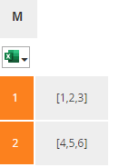
Now consider a matrix M, a list of lists. The datatype of a row of M – let’s call it tMatrixRow – is simply a collection of the FEEL base type Number, and the datatype of the matrix M as a whole – let’s call it tMatrix – is a collection of tMatrixRow. In a matrix, neither the rows nor columns have names. Both rows and columns are referenced by number, i.e., as indices. M[1] means the first row, a list of numbers. M[1][2] means the second column of the first row, a number.
Figure 2. Matrix M, a list of number lists
Working with matrices in FEEL requires iteration, which may be an unfamiliar construct. Iteration in FEEL has two forms both involving the for..in..return construct:
for <<range variable>> in <<list>> return <<expression of range variable>>is called iteration by item value. The range variable is simply a name assigned to an item in the list. The expression following return uses the range variable name wherever the expression involves the list item. Evaluation of the expression generates one item in the output list. So iteration by item value says for each item in an input list generate a corresponding item in the output list.
The other alternative, called iteration by item index, looks like this:
for <<range variable>> in 1..count<<list>> return <<expression of range variable>>.The difference is the term following in is a range of integers from 1 to the number of items in the input list. In this case, the expression uses the range variable as an index.
We use iteration by item value to extract the jth column of matrix M:
for row in M return row[j]Here row is the range variable, an item in the list M. Recall that M is a list of rows, so the range variable row (we could have called it x, or anything) simply means a row of M. And since M is a list of lists, row is also a list. Thus the expression row[j] means return the jth item in the row, i.e. the jth column.
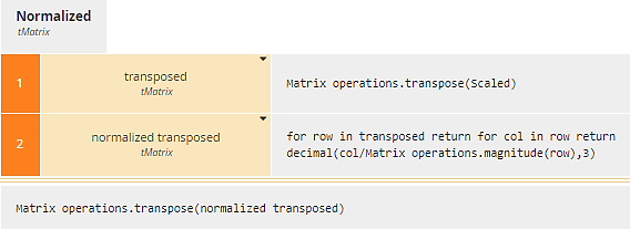
Alternatively, we could have used iteration by item index, as follows:
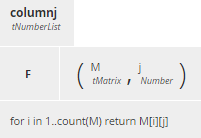
for i in 1..count(M) return M[i][j]Let’s take that apart. Here the range variable i is an integer from 1 to the number of rows in M. The expression M[i][j] means take the ith row of M and then the jth column of that row, iterating over i, i.e., over rows of M. So this also returns the jth column of M.
Matrix Input Data
When using matrices, for the time being there is a minor tool issue we need to deal with. Trisotech DMN Modeler can handle lists of lists internally, but the Execution/Test dialog for entering test data and viewing the results cannot display them. That’s ok. We will enter input data as a relation and convert it to a matrix using the little-known FEEL function get entries(). Get entries maps a data structure, such as a row in our relation, to a two-column table with one row per structure component, the first column key holding the component name and the second column value holding its value. A companion function get value() extracts the value of a selected key in the structure.Matrix Operations Library
When dealing with matrices, it is convenient to call upon a library of basic operations on any mxn matrix, meaning m rows and n columns, or any n-element vector. By clicking Include on the DMN ribbon and selecting the Matrix operations model, you can import BKMs from this model into your own DMN models. They include:- xij(M, i, j), returning the matrix cell value at row i, column j
- dimension(M), returning m, the number of rows, and n, the number of columns
- transpose(M), returning the transpose of the matrix
- column(M, j), returning the jth column of the matrix
- smult(M, a), returning the product of a scalar and a matrix
- madd(M1, M2), returning the sum of 2 matrices with equal dimensions
- mmult(M1, M2), returning the matrix product of two matrices with compatible dimensions
- vmult(V1, V2), returning the dot (inner) product of 2 vectors
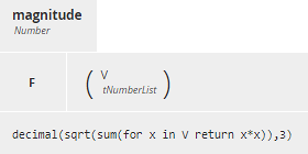
- magnitude(V), returning the root sum squared of the vector elements
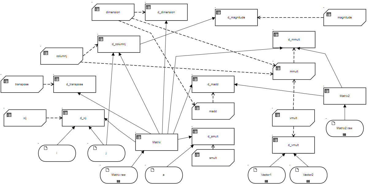
Figure 3. Matrix operations library
The BKMs that map a matrix into another matrix generally rely on nested iterations. These look complicated at first but if you work with matrices you will get used to them. They take the form:
for i in 1..count(M) return for j in 1..count(M[1]) return <<cell value>>The outer for loop iterates over an index to rows of the matrix M. The inner for loop iterates over an index to the columns, modeled as the items in a row of the matrix.
As mentioned earlier, input data can be modeled as a relation and then converted to a matrix using get entries. The decision Alternatives, shown below, converts AlternativesTable, a relation, into tMatrix, a list of number lists:
Figure 4. Conversion of a relation to a matrix
The first context entry AltCriteria generates a list of column names in AlternativesTable, applying get entries to a row of the relation and selecting the component key, returning a list of strings. We don’t want the column Name in our matrix, so we exclude it with a filter. We then iterate over rows of the relation, within each row iterating get value over a list of keys to create the matrix.
Example: TOPSIS
I recently created a model for a client implementing an algorithm for multi-criteria decision making called TOPSIS. You can read more about it here. It can be implemented in DMN either using tables or matrices. I will briefly describe the table implementation and go into more detail with the matrix implementation.Table Implementation
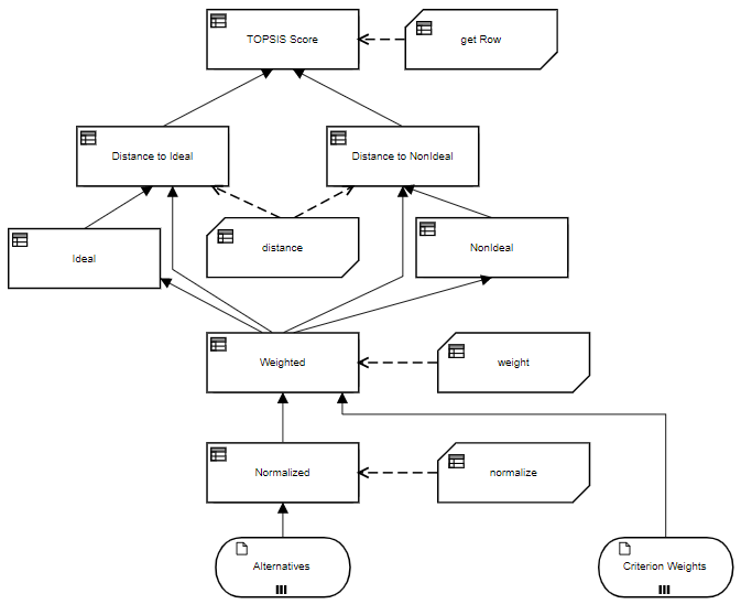
The DRD below illustrates the table implementation.Figure 5. DRD of TOPSIS table implementation
The algorithm basically works as follows:
- You want to compare m Alternatives using n Criteria. Each Criterion contains a rating from 1 to 9, a type, either a Benefit or a Cost, and a weight. For Benefit Criteria, a rating of 9 is best and 1 is worst. For Cost Criteria, 1 is best and 9 is worst. The sum of the weights must be 1. Using tables (relations), each row of input data Alternatives is a structure with a component for each Criterion. The component name is the Criterion name and its value is the rating for that Criterion.
- The Normalized matrix divides each cell value of Alternatives by the root sum squared of the column values.
- The Weighted matrix multiplies each cell value of Normalized by its Criterion weight.
- The vector Ideal is a list of n values representing, for each column of Weighted, the max column value for Benefit types or the min column value for Cost types. The vector NonIdeal is a similar list, but using the min column value for Benefit types and the max value for Cost types. This DRD assumes the decision knows which Criteria are Benefits and which are Costs. Alternatively, you could encode that in the input data Criterion Weights and reference that in the decision logic.
- Each Alternative can be considered a point in n-dimensional feature space, the rating value for each of n Criteria. Ideal and NonIdeal are similarly points in that space. Thus for each Alternative you can calculate the Euclidean distance between it and Ideal, and between it and NonIdeal, where Euclidean distance means the rool sum squared of the difference vector. The decisions Distance to Ideal and Distance to NonIdeal are lists, one item per Alternative, of those distances.
- Topsis Score is a table of m rows, one for each Alternative and its score value,
Distance to NonIdeal/(Distance to Ideal + Distance to NonIdeal).
Values closer to 1 are closer to the Ideal and further from the NonIdeal
Matrix Implementation
To illustrate the matrix implementation, I created an EU-Rent example, a recommender of available rental cars based on the customer’s stated preferences. In addition to allowing any number of Criteria (and adding new ones), it also addresses something that has bothered me about TOPSIS, which is the fact that the Criterion ratings mix objective metrics, like the car’s rental price or miles per gallon, and customer-specific preferences, such as style or number of passengers. My example deals with that, although it could be improved in a couple respects:- More cleanly separate the objective measures – maybe in a zero-input decision – from the customer preferences, which are input data.
- Better map certain objective measures to user preferences. For example, a higher passenger capacity is not necessarily preferred.
DRD
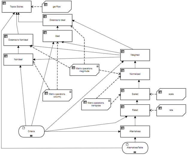
The DRD is shown below. It is similar to the previous one, but inserts two new decisions, Rated and Scaled, between Alternatives and Normalized, and uses BKMs imported from the matrix operations library to deal with common matrix functions.Figure 6. Matrix implementation of TOPSIS
Input Data
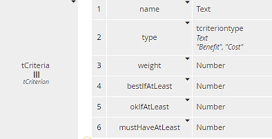
Input data Criteria is a table, collection of tCriterion, shown below. The last three components are used, for certain criteria only, to convert between numeric measures and a rating. For Benefit criteria it makes the assumption that a higher number is better, which is not always the case, so this aspect could be improved.Figure 7. Type tCriteria includes components used in Rated
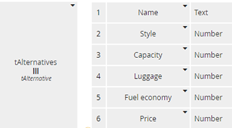
Input data AlternativesTable is also a table for data entry purposes, but it will be mapped to a matrix. Each row of AlternativesTable is a structure containing its Name and scores on various criteria.
Figure 8. Type tAlternatives models input data as a relation
Alternatives
Decision Alternatives maps AlternativesTable to a matrix, type tMatrix, a list of number lists. As shown earlier, it uses the FEEL functions get entries and get value. Because get entries does not return the list of components in the same order as the structure definition, we need to use the values of the column Criteria.name as the key name in get value. This ensures the order of the columns in the matrix matches their order in input data Criteria.Figure 9. Alternatives maps the list of delimited strings to a matrix
Rated
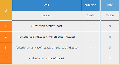
Decision Rated maps certain cells of Alternatives to a rating based on customer preference by calling the BKM rate. The mapped cells are those for Criteria with a non-null value in component bestIfAtLeast. The BKM rate compares the cell value to the values of components bestIfAtLeast, okIfAtLeast, and mustHaveAtLeast with the assumption that more is better. The logic of this BKM is not the best; it should be improved.Figure 10. Rated maps some raw Criteria values to rating based on user preference
Figure 11. BKM rate implements the preference mapping
Scaled
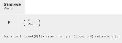
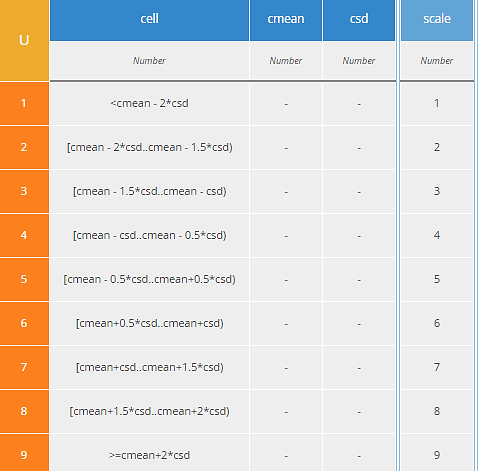
Decision Scaled is a departure from “official” TOPSIS in that it rescales the value of any Criterion to a range from 1 to 9 using the mean and standard deviation across all Alternatives. A value equal to the mean is assigned a rating of 5. A value 2 standard deviations higher is assigned a rating of 9, and a value 2 standard deviations lower is assigned a rating of 1. Values in between are interpolated and rounded to the nearest integer. Values beyond 2 standard deviations from the mean are clipped at 9 or 1.Scaled is a context that makes use of the matrix operation transpose. The first context entry columns transposes Rated, making it a list of columns. Context entry scaled columns iterates over that list, calling the BKM scale, with arguments the cell value, the column mean, and the column standard deviation. This is a simple decision table. The reason it has columns for the mean and standard deviation is that for a BKM, the parameters are specified by the input column names. Yes, stupid, I know. It’s in the spec. The final result box uses transpose again to put the matrix back in proper order.
In my implementation, I applied scaling even to Criteria values that are manually rated. That is probably incorrect. An improved implementation would apply scaling only to objective Criteria values.
Figure 12. Scaled uses transpose twice to operate on columns of Rated
Figure 13. BKM Matrix operations.transpose
Figure 14. BKM rate implements the scaling algorithm
Normalized
Decision Normalized, from the original TOPSIS algorithm, divides each cell in Scaled by the root sum squared of its column values. Since a column of the matrix is a vector, we use the imported Matrix operations.magnitude function to calculate that. As in Scaled, we use Matrix operations.transpose to work on columns and then transpose back again.Figure 15. Normalized uses transpose twice to operate on columns of Scaled
Figure 16. Matrix operations.magnitude calculates the root sum squared of a vector
Weighted
Decision Weighted applies customer-selected weights to each Criterion. The weights must total 1.0.Figure 17. Weighted multiplies each cell of Normalized by the Criterion weight
Ideal and NonIdeal
Decision Ideal calculates the list, one element per Criterion, representing the maximum value of Weighted for Benefit Criteria or the minimum value for Cost Criteria. NonIdeal is the same but swapping Benefit and Cost. For n Criteria, Ideal and NonIdeal can be thought of as vectors in n-dimensional feature space.Figure 18. Ideal selects the max Weighted value for Benefit Criteria, min value for Cost Criteria
Figure 19. BKM Matrix operations.columnj extracts the jth column of a matrix
Distance to Ideal, NonIdeal
Each row of Weighted – corresponding to a different Alternative – can similarly be envisioned as a vector in the same n-dimensional feature space. Decision Distance to Ideal calculates, for each row of Weighted, the Euclidean distance between that row vector and the Ideal vector, applying Matrix operations.magnitude to the difference vector. Decision Distance to NonIdeal does the same, substituting the NonIdeal vector for Ideal.Here Distance to Ideal is modeled as a context. Each row of context entry deltaMatrix is the difference vector between the corresponding row of Weighted and Ideal. The final result box calculates the magnitude of each difference vector. Distance to NonIdeal is the same, substituting NonIdeal for Ideal.
Figure 20. Distance to Ideal computes the difference vector between each row of Weighted and Ideal, then calculates the magnitude of that difference vector.
TOPSIS Scores
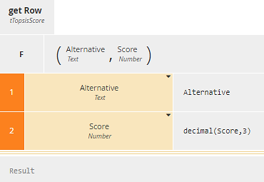
For the top-level decision Topsis Scores we want a table that lists each Alternative by name along with its Score, calculated as Distance to NonIdeal/(Distance to Ideal + Distance to NonIdeal), and sorts the list in decreasing score order. Context entry unsorted iterates over each Alternative to call BKM get Row, which simply formats a row of the table output. The final result box uses the FEEL sort function to list Alternatives in decreasing score order. The second argument of sort is always a boolean function of two range variables - here x and y. A true value means x precedes y in the sorted list, so x.Score>y.Score means the list is sorted in descending order of the component Score.Figure 21. Topsis Scores calculates the score for each Alternative, then sorts the list
Figure 22. BKM get Row simply formats rows of Topsis Scores
EU-Rent Example
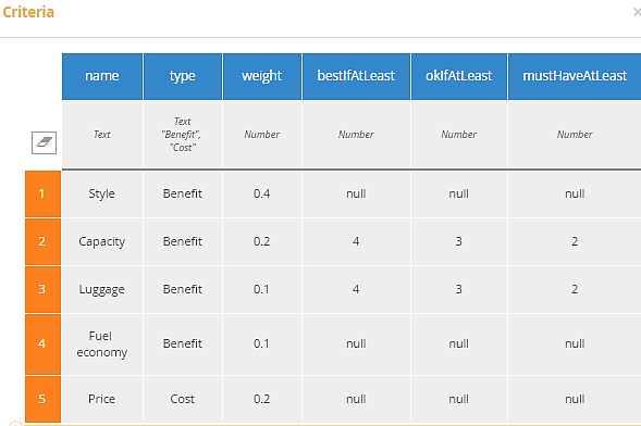
As an example, consider a rental car recommendation decision for EU-Rent. In this example, we consider Criteria to include 5 attributes, as shown below in Execution/Test:Figure 23. Rental car selection Criteria
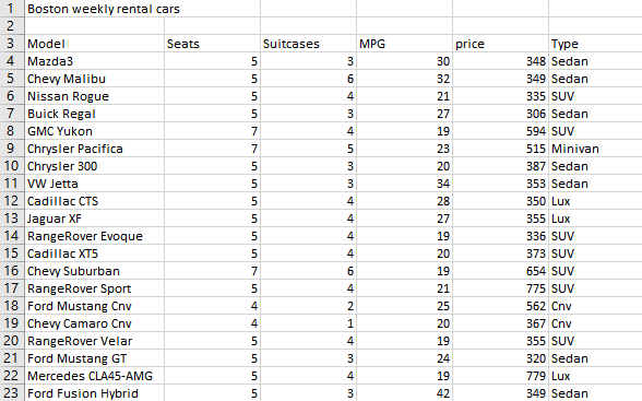
Figure 24. Raw rental car data, BOS weekly rental, hertz.com
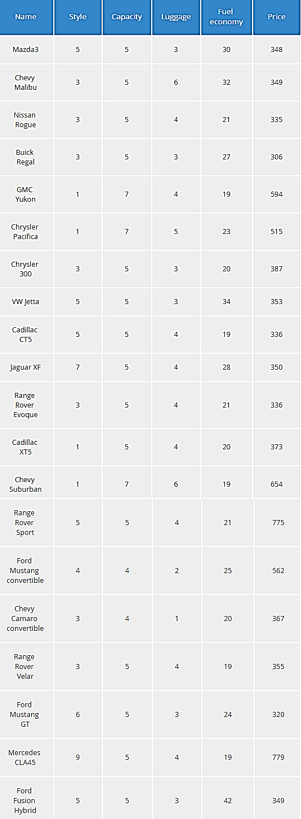
“Objective” values, taken from hertz.com weekly rental in October at Boston Logan Airport, include Fuel Economy (MPG) and Price. Capacity (Seats) and Luggage (Suitcases) are “semi-objective” in the sense that the customer might not always rate a higher value as preferable. For the semi-objective attributes, Criteria asks the customer to provide values for bestIfAtLeast, which gives a rating of 9; okIfAtLeast, a rating of 6; and mustHaveAtLeast, a rating of 3. As noted previously, this logic is not the best, as a customer might rate a car seating 5 higher than one seating 7. The purely subjective attribute Style is selected by the customer as the first scoresText entry in input data Alternatives Raw:
Figure 25. Input data AlternativesTable in Execution/Test
These values are saved as Test Case 1. To run the model with these values, in Execution/Test click Load and select Test Case 1. Running the model gives the following sorted Topsis Scores, with Jaguar XF being the top rated. A customer giving a higher weight to Price would likely have a different recommendation.
Figure 26. Topsis Scores output in Execution/Test
Improving the Model
The model could certainly be improved by better separating purely subjective criteria like Style, from semi-objective criteria like Capacity and Luggage and purely objective criteria like Fuel Economy and Price. I think best if the purely objective ones are not input data at all but a zero-input decision and the semi-objective ones use a better mapping of the raw numeric values to a customer rating from 1 to 9. Also, it’s probably better to apply scaling only to the objective measures, since the others are already in a 1-9 range.Readers are invited to make those improvements and send them to me. We will post the good ones on the site.

